What do I do with my numbers at the end of the month? What am I looking for? What are the numbers showing me? What do I need to do to set my spending plan spreadsheet up efficiently and effectively for the next month? I’ll dive into some of these questions and share with you a few techniques that I have learned from “doing my numbers” regularly for a few years now.
Writing this, it is October 31st and tomorrow begins a new month. I am at the end of my spreadsheet and need to lay out the upcoming month. I have tried various ways to do what I’m about to attempt to explain but this is the quickest way to get up and going for next month’s spending plan. When the Daily Spending Plan columns run out because the month is over, the last column in the spreadsheet should be that month’s total. For me, it says “Oct Total Actual”. That means at the end of the month, these were my actual totals of each category line item for the whole month of October.
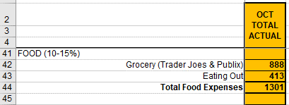
I’ll scan down this totals column and look to see if any number stands out as being higher or lower than normal. I might double check a formula or two to ensure they are working correctly. I’m looking to see if any of the numbers seem a little off. At the same time, I’m also taking a quick mental assessment of: Ok, I spent $888 this last month on groceries, $413 on eating out. That ratio seems higher on the eating out amount than in past months. We must have eaten out more this last month than cooking at home.

I’m really able to compare that better to previous month totals and the averages when I put them into the Monthly spreadsheet. See below. I’m more than double our average for eating out in October. Wow.

I then scroll over to the first column of the month. I grab with my mouse the top left cell, then I highlight everything that I want to copy over to the next month, so I’ll select all the way to the bottom right-hand corner of the daily spending plan for that month. Once highlighted, I right click inside the area and select “copy” or Cntr V. Then I’ll go past the last column (Oct Total Actual) and skip a column but then right click on the spot where I want the top right-hand corner of the next month to start. Right clicking there and selecting “paste”, or “Ctrl P” the entire month for October just copied over to set up the template for November.
Because I color code each day as I complete each day’s numbers, the entire month for October was colored orange. I need to now highlight the entire area that I just copied and select “no fill” for the color. That will remove the coloring, setting it up to be a blank slate for the new month.
Before we go much further, let’s stop and discuss what we just did. We successfully just copied and pasted all the formulas and expense details from last month over to this new month. That is crucial because when I’m in the new month, I want to see for example, what day last month did I pay the house bill…so that I can pay it around the same time this month. I want to see when my gym monthly membership goes through so that I can see that coming and make sure I have enough in the account before that clears the bank. It is a rough spending plan from last month’s actuals that I’ll use to help facilitate spending in this upcoming month.
Next, I go through and change the days of the weeks. I leave the numbers 1-31 because those won’t change. There are still 1-30 or 31 days in the following month. All I change is the part that says FRI, SAT, SUN, MON, etc.

I click on the date and time at the bottom right of my screen to pull up a small calendar. It tells me that the first is a Monday. October’s first day of the month was Friday. November’s first day of the month is Monday. So quickly go through and manually change FRI to MON, then the 2nd will say TUE, 3rd will say WED…all the way to the end of the spreadsheet.

I’ll pull back up that calendar to just check to see what day the last day of the month lands on. For November, it lands on a Tuesday and there are only 30 days in that month. I simply hide the extra 31ST day column so that it will be there for when I copy it over again to lay out December…because December has 31 days in the month. Hiding a row or column should NOT mess up the formulas.
Now that we have the days of the month in-lined with the correct columns, I want to make sure to explain clearly that I like to leave the spending historical data in the cells for what I spent last month. That helps me to plan out what I will most likely spend this next month.
However, with the time tracking, I go ahead and clear out that area so that it is prepped for the next month.

Every cell gets cleared except for the sleep area, that formula will be reset to clear out the hours from when I went to bed to midnight for that night.
Daily time tracking for the last 24 hours has just become another quick step in doing my daily numbers. I don’t spend more than 3 mins on it…if that. I simply think back to what happened the following day. I made an estimate on how much time I spent with my family…How much time spent on selfcare…How much time did I spend doing service, having fun doing my hobbies? That’s it. It is not an exact science. I’m probably about 80% accurate and that is ok. The only category that I want to be as accurate as possible is tracking my time working for my job. The main goal is that I can tell if I’m over or under working, or right on track.
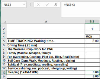
It is important to only clear out one week’s time tracking section at a time to not mess up the formulas that are in place. Select the Waking Time cell and highlight all the way to the bottom right cell in that week, landing on sleeping. When they are highlighted, hit delete. Also, while they are highlighted, right click in the center of that area, and hit “Delete Note” and that will clear out any notes. Then continue clearing out the time tracking sections week by week until the end of the month. We will go back in and add in the sleeping formula at the end. It’s a simple step, but helpful and a time saver. Please note that the bottom line in the time tracking section is a total of that day’s hours (row 14 in the chart above). Be careful to not clear out that total or else we will have to recreate it. The daily total hours should add up to 24 hours or more for each day.
Now go back to the first day of the month for November. Click in the cell for the row that says sleeping. Click = then simply use the mouse to select the “wake up time” cell for that day…then hit enter. The way I track my time for sleeping is I account for the hours from midnight to midnight for that day. This is the key point that I realized early on in tracking my time.
How do you handle tracking the hours slept? It’s from midnight to the time that I woke up, plus the hours I went to sleep until the next midnight. For example, when I’m doing my numbers and thinking back on the following day, all I must think about is what time I went to bed last night. If I went to bed at 9pm, that is 3 hours that I need to add to my awake time for yesterday. If I woke up at 5am yesterday, in the cell where we have sleeping, I’m simply going to click into that formula and add +3 behind the existing formula which will show sleeping was 5hrs (from midnight to 5am) + 3hrs (from 9pm to midnight) = 8 hours of sleep for yesterday. PERFECT! I try to hit 7.5-8hrs of sleep daily and time tracking helps me know if I’m hitting that goal or not. Watching how I do this in my upcoming video might be a whole lot easier to follow. Stay tuned for that video.

Notice the formula says =NS5+3. I woke up at 5am and went to bed at 9pm = 8 hours of sleep for that day.
Lastly, I’ll go through and change the “OCT WK 1 Total” header to say, “NOV WK 1 Total” and do that for the 5 weekly totals.

change to

I also clear out the last line in the daily spending plan spreadsheet titled Daily Account Balance. That entire can be highlighted all the way for the new month and then hit Delete to clear all the totals. That balance is important because it causes me to register in my mind how much cash is in my checking account. I can make a mental note in case there are some bills or checks outstanding that haven’t gone through yet. If I have $100 in my checking account as the ending balance when I’m doing my numbers, but I can see that tomorrow is the day that our power bill is clearing the bank and it is $200, then I realize that I need to transfer some money.

And that is it. We are all set up with our spending plan template for next month. To utilize the data from the month I just completed, I will take the final column totals and put them into the monthly PRG Dashboard spreadsheet. I’ll cover that in a future writing.
There I’ll be able to compare income, spending, debt repayment, and savings plans on a month-to-month basis. That is how I close out a month like last October and set up my spending plan for the new month. I will have this in a video format soon which might be easier to follow.
To check out last week’s newsletter, you can find it here: https://pathtowarren.com/checklist/
To listen to Podcast Episode 260 where we discuss Advanced Time Tracking: How to Capture Sleep:
To listen to Podcast Episode 139: Time-Drunk
Remember to “Make your contribution”, as mama always says.
Thanks for letting me share. – Matt


